Data files can be downloaded from this page or requested from the author. Please send me email : irina@geo.ku.dk indicating which data you are interested in and for which region. |
| Global 1°x1° thermal model TC1 for the continental lithosphere: Implications for lithosphere secular evolution |
Surface heat flow measurements allow us to constrain the thermal
state of the upper mantle only for about 40% of the continents (Figure
1), which is sufficient to perform a statistically significant analysis of
lithospheric geotherms for continental terranes with different tectonic
settings and different geological ages. New compilation of crustal
ages (Figure 2) together with previously reported geotherms for
stable continental regions (Artemieva and Mooney, 2001) form the
basis for this analysis. These data were supplemented by xenolith
P-T arrays and electrical conductivity profiles for cratonic regions. A
new global thermal model TC1 for the continental lithosphere is
constrained on a 1ox1o grid.
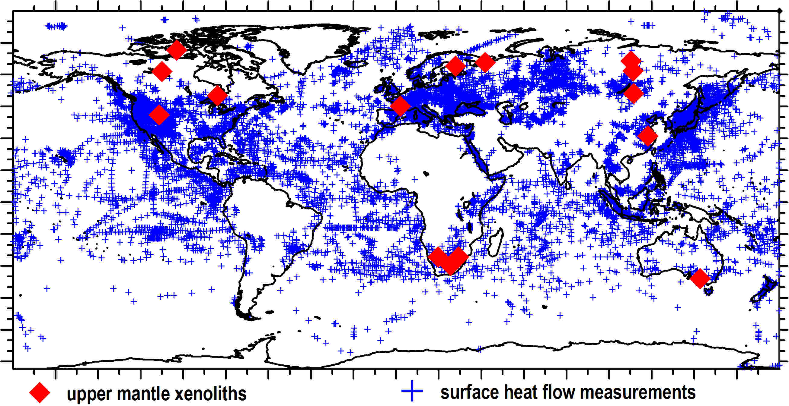
| Figure 1. Global heat flow data coverage (updated after Pollack et al., 1993). Crosses – sites of borehole heat flow measurements; diamonds – locations of mantle xenoliths discussed in the text. |
Global 1 deg x 1 deg compilation of tectono-thermal ages of the continental lithosphere

| Figure 2. Geological ages of the continents on a 1ox1o grid (based on Goodwin, 1996; Fitzgerald, 2002; Condie, 2005, and numerous regional publications). The map shows the ages of the major crust-forming events (see Table 2), rather than ages of the juvenile crust, and forms the basis for the global thermal model for the continental lithosphere TC1. Note: this map can be slightly different from the published one due to on-going updates of the database. |
A major assumption for the analysis is that
lithospheric mantle has the same age as the
overlying crust.
Statistical analysis of continental geotherms constrained by heat flow data

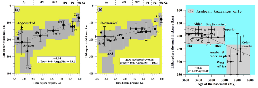
| Figure 4. Correlation between lithospheric thermal thickness and geological age of terranes. The bars indicate the scatter in the values, but not their uncertainties. (a) Global correlations for continents based on individual heat flow measurements; gray area shows the general trend of lithospheric thickness variations with age (Artemieva and Mooney, 2001); (b) Global correlations for continents, area-weighted on a 1ox1o grid for terranes of different ages; (c) correlations for Archean terranes; abbreviations: Ar=Aravalli, Dhw=Dharwar, K=Kaapvaal, Pilb=Pilbara, Yi=Yilgarn, Z=Zimbabwe cratons, Ukr=Ukrainian shield. Data for the Slave craton is not shown because only one heat flow measurement exists. Archean cratons are subdivided into three groups (Figure 2 and Table 2): Ar-I includes cratons formed at 3.0-2.5 Ga, Ar-II includes mostly cratons of Gondwana-continents with basement ages >3.0 Ga, Ar-III includes cratons reworked by Phanerozoic tectono-magmatic events (e.g. Sino-Korean, Wyoming, Tanzanian and Congo cratons). |
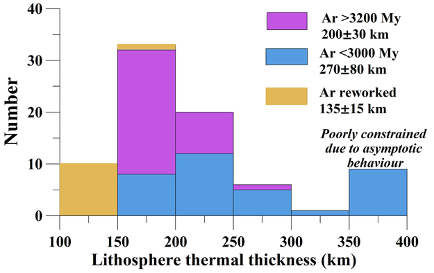
| Figure 3. Statistics of lithosphere thermal thickness based on heat flow data estimates (point data); (upper) Proterozoic-Paleozoic terranes; (lower) Archean terranes. |
regime (Figure 4a): the lithospheric thermal thickness linearly decreases with time from Mesoarchean to present. However, this
correlation can be biased by the uneven distribution of heat flow measurements as indicated by the lower value of area-weighted
correlation (r=0.68) calculated on a 1ox1o grid (Figure 4b).
2) Contrary to the global trend, lithosphere is thicker in young Archean than in old Archean (>3.0 Ga) cratons (Figure 4c). Thick
lithospheric roots (250-350 km) are found solely for 3.0-2.5 Ga cratons. In several Archean cratons regions with low heat flow, thick crust
and thick lithosphere spatially coincide with paleoterrane boundary(ies). I propose that in such regions an exceptionally thick lithosphere
has a relatively small lateral extent and was formed during Archean-early Proterozoic thrust-thickening collisions of pre-existing
continental nuclei. Heat from the mantle during episodes of high tectonic activity could be effectively diverted by such “lithospheric teeth”,
forming belts of anorogenic magmatism at their edges.
3) A map of tectono-thermal ages of lithospheric terranes complied for the continents
on a 1ox1o grid (Figure 2) and combined with the statistical age relationship of continental
geotherms (z=0.04*t+93.6, where z is lithosphere thermal thickness in km and t is age in
Ma) (Figure 4) formed the basis for a new global thermal model of the continental
lithosphere (TC1).
on a 1ox1o grid (Figure 2) and combined with the statistical age relationship of continental
geotherms (z=0.04*t+93.6, where z is lithosphere thermal thickness in km and t is age in
Ma) (Figure 4) formed the basis for a new global thermal model of the continental
lithosphere (TC1).
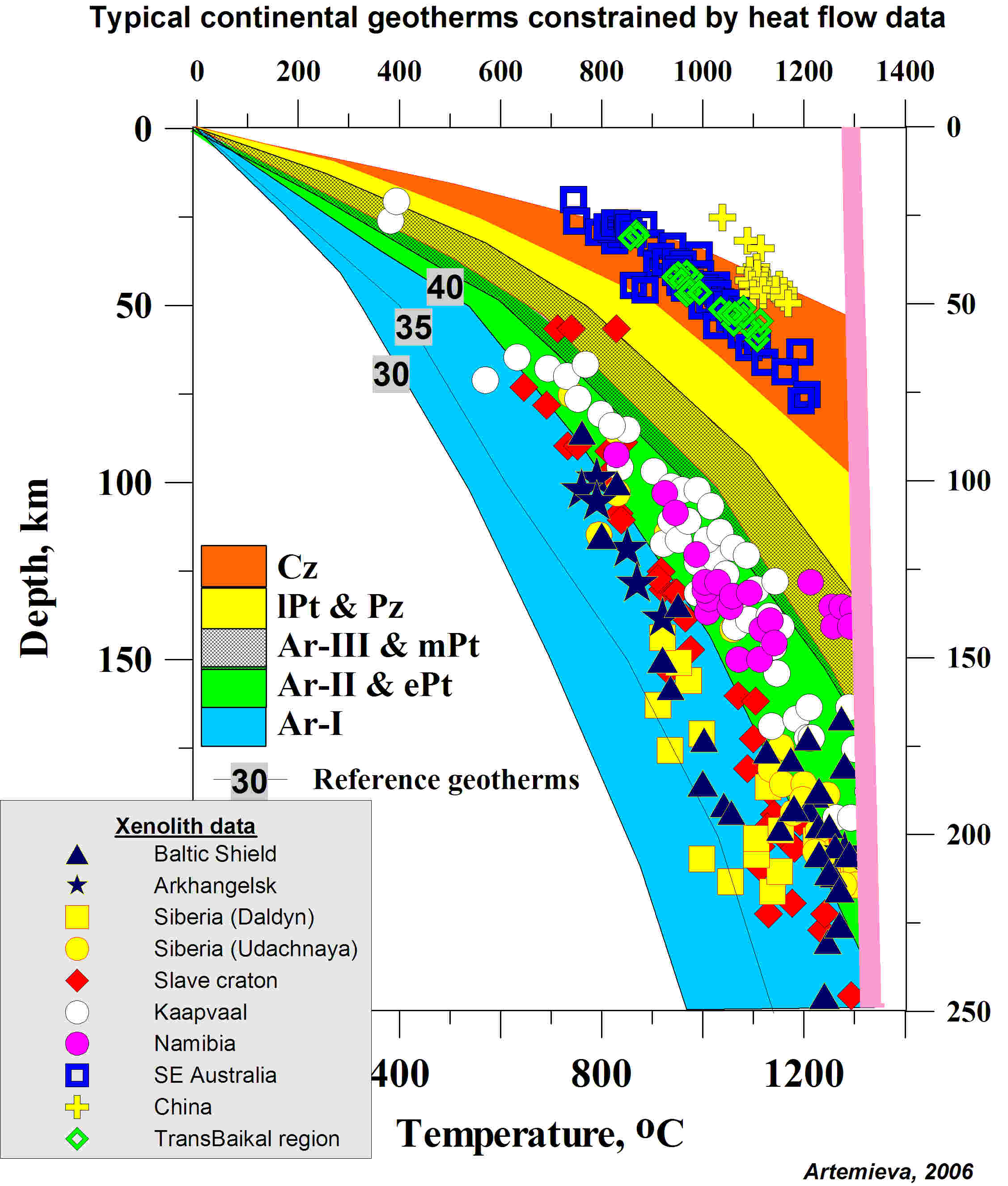
| Figure 5. Typical continental geotherms constrained by heat flow data for stable regions and by xenolith data for active regions. Five groups of typical geotherms include (from the coldest to the warmest):
flow in mW/m2. |
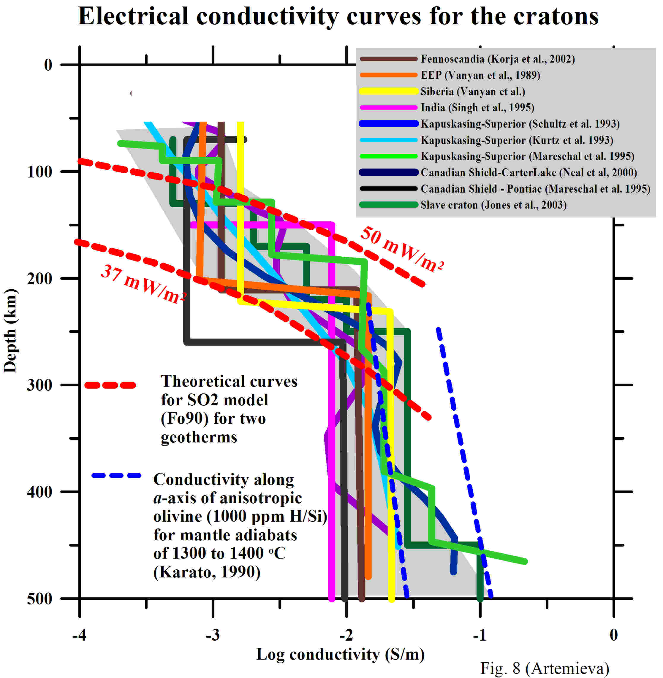
4) Xenolith P-T arrays confirm the results of the thermal model and suggest that there are two groups of Archean cratons with
significantly different thermal regimes. Cratons with lower mantle temperatures follow a ca. 35-38 mW/m2 conductive geotherm and include
Archean terranes of the northern hemisphere (Slave craton, Fennoscandia (central Finland and Arkhangelsk region), and Siberia).
Xenolith P-T arrays for Kaapvaal, Namibia, Superior and Wyoming cratons, and Somerset Island follow a 40-45 mW/m2 conductive
geotherm. The difference between the 37 and 42 mW/m2 geotherms implies ca. 80-100 km difference in the lithospheric thickness between
the cratons in the two groups. Depth curves of electrical conductivity, which are surprisingly similar for all cratons, further support the
conclusion that conductive geotherms between 35 and 50 mW/m2 are characteristic of all of the Archean cratons.
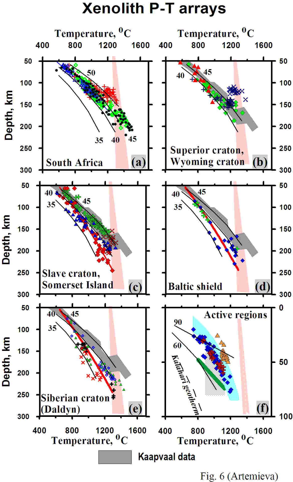
| Figure 6. Xenolith geotherms for continents clearly indicate two typical cratonic geotherms: ~45 mWm2 (a, b) and ~37 mWm2 (c-e). Because xenolith P-T arrays constrained by different geothermobarometers are significantly different, the data are shown mostly for the BKN method (Brey, Taylor, 2000), MC (MacGregor, 1974), FB (Finnerty and Boyd, 1987) and ONW (O’Neill and Wood, 1979). Thin lines – conductive geotherms of Pollack and Chapman (1977), values are surface heat flow in mW/m2. Pink shading – mantle adiabat. (a) South Africa: blue triangles – Kimberly (Kaapvaal), green rhombs – Lesotho, red crosses – Gideon, Namibia (all three BKN-NT data from Grutter and Moore, 2003); black circles – xenolith data from several locations in Kaapvaal (compilation of Rudnick and Ny¬blade, 1999); these data are shown in plots (b-e) by gray shading; (b) Superior craton (Kirkland Lake) - green rhombs (data from Pearson et al., 1998); Wyo¬ming craton - blue pluses (NT-NT data from Pizzolato and Schultze, 2003) and blue crosses (BKN data from Hearn, 2003); red triangles –SW Arkansas (BKN data from Dunn et al., 2003); (c) Slave craton: red rhombs – low-T peridotites (red lineshows the best-fit) (BKN data from Kopylova et al., 1999; Kopylova and McCammon, 2003), red crosses – high-T peridotites (BKN data from Kopylova and McCammon, 2003); blue triangles – Lac de Gras area (BKN data from Menzies et al., 2003); green pluses – Somerset Island (MC-NT data from Grutter and Moore, 2003); (d) Fennoscandia: blue rhombs - central Finland (BKN data from Kukkonen and Peltonen, 1999; Lehtonen et al., 2003); green crosses – Arkhangelsk, pipe Grib (BK-MC data from Malkovets et al., 2003); red line – best fit for the Slave craton; (e) Siberian craton (Daldyn terrane): blue rhombs and green triangles (correspondingly, FB and ONW data from Griffin et al., 1996); black pluses – Zarnitsa pipe, red crosses – Irelyakhskaya pipe (both NT-NT data from Aschepkov et al., 2003); (f) active regions: orange triangles – SE China (data from Xu et al., 1996); blue diamonds – SE Australia (data from O’Reilly and Griffin, 1985); red crosses – Tariat region, Mongolia (data from Ionov et al., 1998); blue shading – Baikal region: Sayans, Vitim, and Udokan (data from Litasov et al., 2003); green line – Rhenish massif (after LeBas, 1987); hatched area – Massif Central (after Coisy and Nicolas, 1978; Masse, 1983); for a comparison a typical Kalahari geotherm is shown by dashed line (Rudnick and Nyblade, 1999). Note different depth scale of the plot. |
| Global correlations between thermal regime of the continental lithosphere, xenolith geotherms, and electrical structure of the cratonic upper mantle |
GLOBAL THERMAL MODEL FOR THE CONTINENTAL LITHOSPHERE TC1
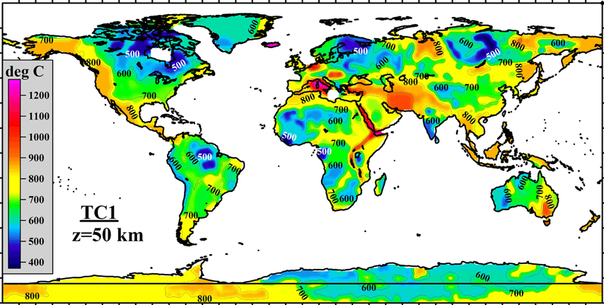
| Figure 10. Global thermal model for the continental lithosphere TC1 constrained on a 1ox1o grid: temperature at a 50 km depth interpolated with a low-pass filter. |
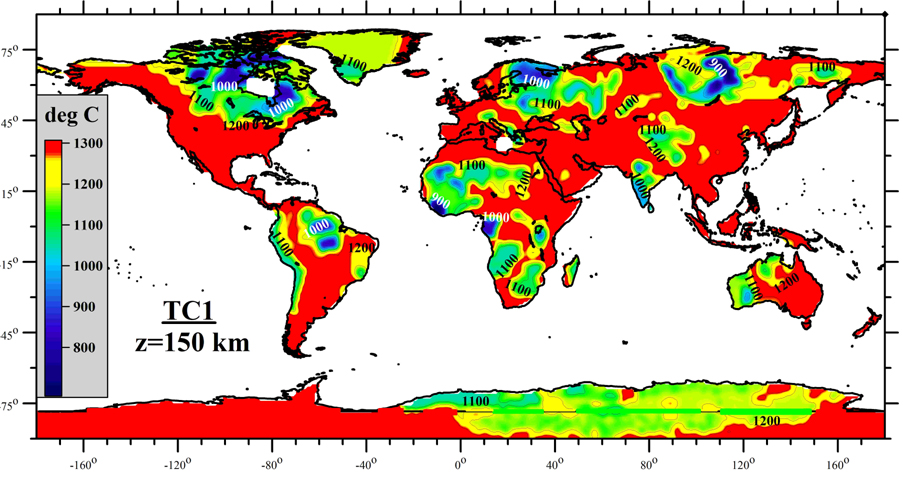
| Figure 11. Global thermal model for the continental lithosphere TC1 constrained on a 1ox1o grid: temperature at a 150 km depth interpolated with a low-pass filter. |
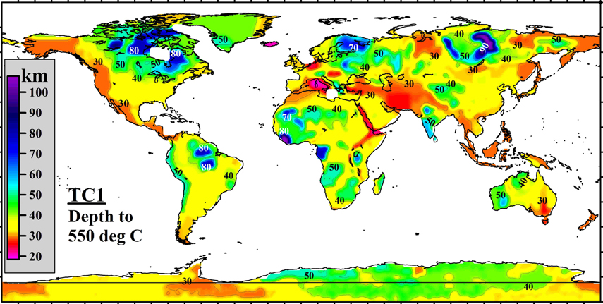
| Figure 13. Global thermal model for the continental lithosphere TC1 constrained on a 1ox1o grid: depth to the 550 oC isotherm interpolated with a low-pass filter. This depth can be considered a proxy of the thickness of magnetic crust (Petersen and Bleil, 1982) and as a proxy of the depth to the brittle-ductile transition in mantle olivine (Kusznir and Karner, 1985). |
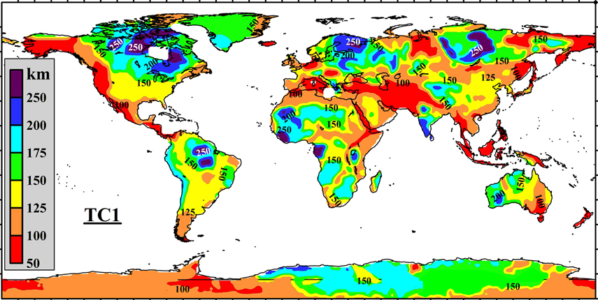
| Figure 12. Global thermal model for the continental lithosphere TC1 constrained on a 1ox1o grid: lithospheric thermal thickness interpolated with a low-pass filter. The values are based on typical continental geotherms (Figures 3-6) and the age of the basement (Figure 2). |
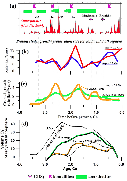
1) A global map of lithospheric thickness (Figure 12), constrained by the TC1 model, was used to estimate the volume of the preserved
continental lithosphere, which is ca. 27.8(± 7.0)x10^9 km3 (excluding submerged terranes with continental crust such as oceanic plateaus and
shelves). The average growth rate of the continental lithosphere was ca. 5-8 km3/year in the Archean and twice higher at 2.1-1.7 Ga. About
50% of the present continental lithosphere was formed by 1.8 Ga.
2) The growth rate of the lithosphere since the Archean (as manifested by its present-day lithospheric volume for terranes of different ages)
(Figure 15b) does not reveal a peak in lithospheric volume at 2.6-2.7 Ga as expected from growth curves for juvenile crust (Figure 15c). A
nearly zero rate of lithosphere recycling (Figure 15d) was calculated for the Archean-early Proterozoic lithosphere, reflecting stabilization of
cratonic lithosphere by the late Archean and its enhanced survivability.
3) The major peak in the rate of lithospheric growth correlates with one of the major world-wide recognized crust-forming episodes at 2.0-1.7
Ga and is followed by a global extraction of Proterozoic massif-type anorthosites. I propose that large-scale variations in lithospheric thickness
at cratonic margins and at paleoterrane boundaries controlled anorogenic magmatism and, in particular, the extraction of Precambrian
anorthosites which were produced by vigorous small-scale convection at the margins of continental lithospheric keels formed at 2.0-1.7 Ga.
The hypothesis is based on the observed correlations (a) between the spatial distribution of Proterozoic anorthosites and lithospheric
structure and (b) between the time of their extraction and lithosphere growth rate. More common and more voluminous occurrence of middle
Proterozoic massive anorthosites in the northern hemisphere (where xenolith and thermal data suggest an exceptionally thick lithosphere)
supports the hypothesis that their emplacement can be associated with a presence of >250 km lithospheric roots.
| Last modified June 24, 2006, irina@geol.ku.dk |
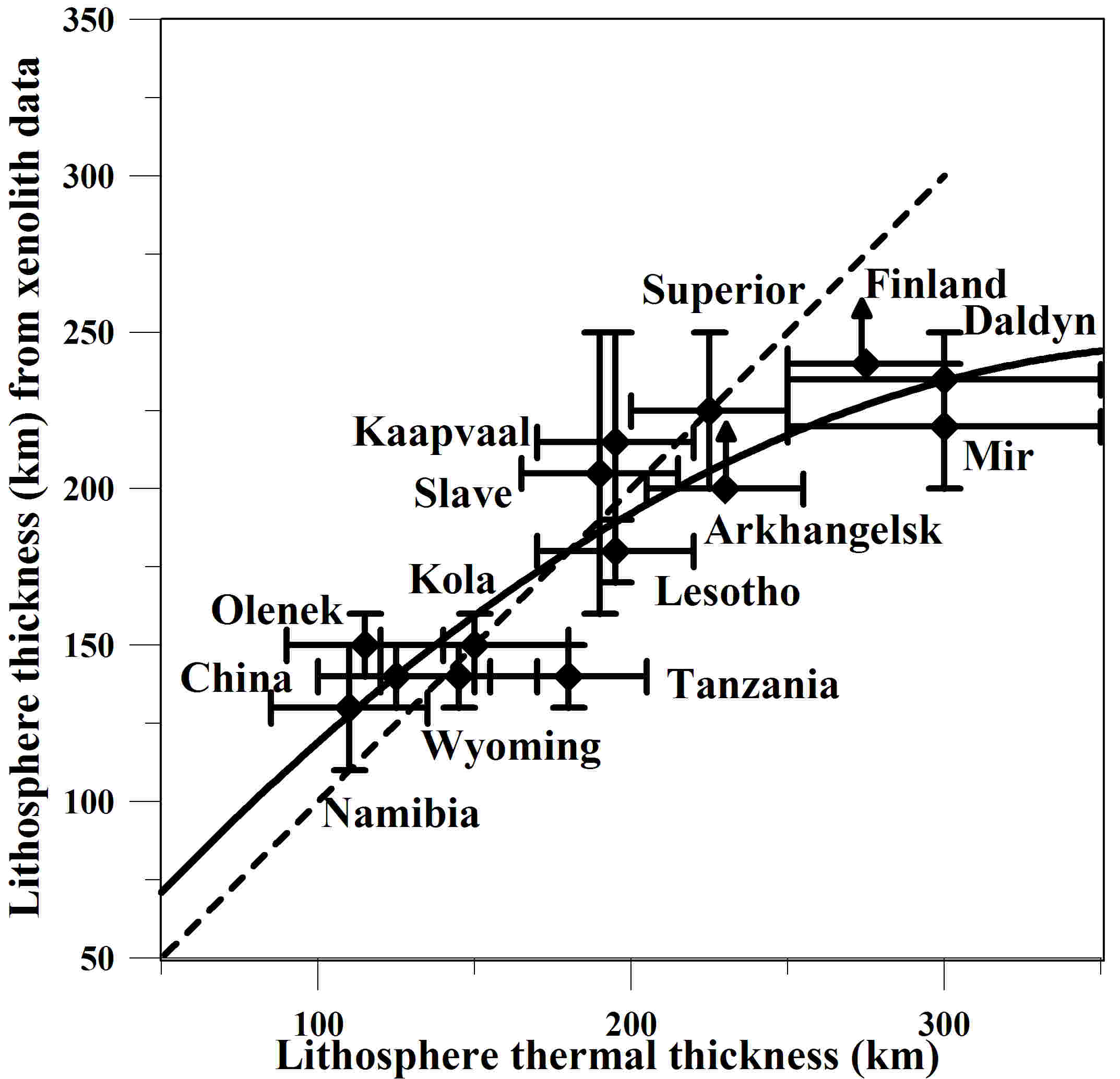
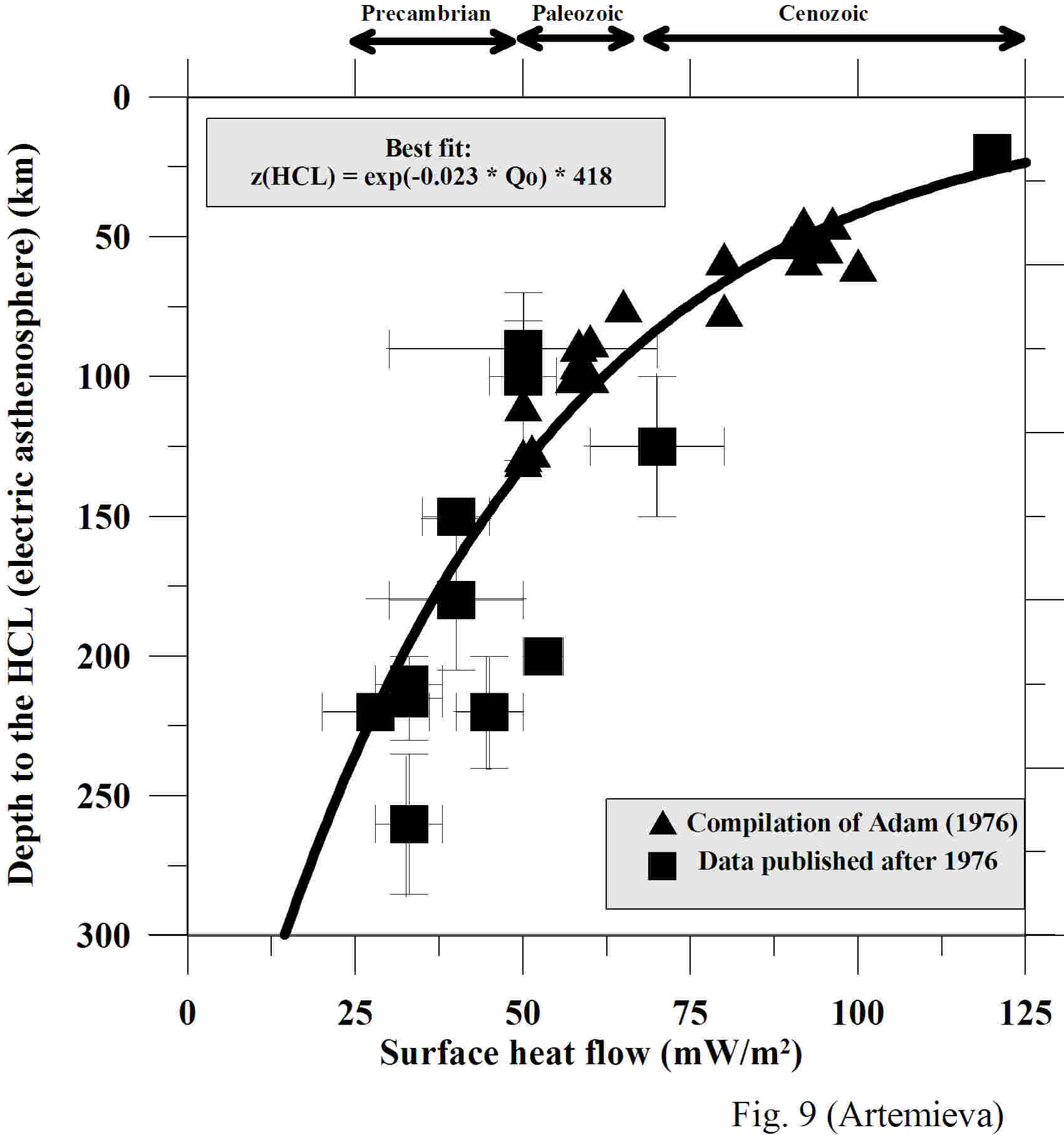
| Figure 7. Correlation between lithospheric thickness constrained by heat flow and xenolith geotherms for stable continental terranes. Note that the bars show the range of thickness estimates for different cratonic blocks, but not an uncertainty. Because the deepest known kimberlite magmas originated at ca. 250 km depth, xenolith and thermal constrains on lithospheric thickness diverge at greater depth. However, xenoliths from Finland derived from 240 km depth do not show shearing and suggest lithospheric thickness greater than 240 km (shown by an arrow). Figure 8. Electrical conductivity profiles for different cratonic regions of the world: Baltic shield (Korja, 1993; Korja et al., 2002), East European craton (Vanyan et al., 1977), Ukrainian Shield (Zhdanov et al., 1986), Siberia (Safonov et al., 1976; Vanyan and Cox, 1983; Singh et al., 1995), India (Singh et al., 1995), Slave craton (Wu et al., 2002; Jones et al., 2003), and Superior Province (Schultz et al., 1993; Kurtz et al., 1993; Mareschal et la., 1995; Neal et al., 2000). Also shown are synthetic conductivity curves calculated for conductive continental geo¬therms of 37 and 50 mW/m2 for the standard olivine model SO2 (Constable et al., 1992) with 90% of forsterite (thick solid lines) and conductivity along a-axis of anisotropic wet olivine (1000 ppm H/Si) for mantle adiabats of 1300 to 1400 oC (Karato, 1990) (thick dashed lines). It is important to note that all cratonic conductivity curves fall between theoretical conductivity estimates for 37 and 50 mW/m2 conductive geotherms, in agreement with thermal (Figure 5) and xenolith (Figure 6) constraints. Figure 9. Correlation between surface heat flow and depth to the high-conductive layer in the mantle (electric asthenosphere). Depth to HCL is based on interpretations of Adam (1976), Adam and Wesztergom (2001), Bahr (1985), Berdichevsky et al. (1980), ERCEUGT-Group (1992), Jones et al. (2003), Korja (1993), Kurtz et al. (1993), Mareschal et al. (1995), Moroz and Pospeev (1985), Safonov et al. (1976), Schultz et al. (1993), Simpson (2002), Singh et al. (1995), Vanyan and Cox (1983), Zhdanov et al. (1986). The curve can be used as a proxy to the depth of the HCL for regions with a known heat flow. |
The strong correlation between the thermal state and the age of the lithosphere allows us to build a new global thermal model TC1 of
the continental lithosphere on a 1ox1o grid, which shows strong thermal heterogeneity of the continental mantle. Maximum temperature
anomalies (up to 800 oC) in shallow mantle can produce seismic velocity anomalies of up to 3%. A map of the depth to the 550 oC
isotherm provides a proxy for the thickness of the magnetic crust and for the thickness of a mechanically strong layer in >200 Ma
lithosphere with olivine rheology of the mantle.
Artemieva I.M.
Tectonophysics, 416,
245-277, 2006.
Tectonophysics, 416,
245-277, 2006.
| Growth and preservation rate of the continental lithosphere; correlation with global tectonic events |
| Figure 15. Growth, preservation, and recycling of the continental lithosphere. (a) Timing of global tectonic events: superplumes, komatiite extraction, giant dike swarms (GDS) (after Condie, 2004, 2005), and Archean and Proterozoic anorthosites (data from Ashwal, 1993). (b) Growth/preservation rate of the present-day continental lithosphere (crust + lithospheric mantle) calculated on a 1ox1o grid from the global model of lithospheric thickness TC1 (Figure 12) with age steps of 0.2 Ga (black line) and 0.3 Ga (gray line). The peak in lithospheric growth at ca. 1.7-2.0 Ga is a robust feature of the model. Note that this peak is followed by massive extraction of Proterozoic anorthosites suggesting that they were produced by edge-driven convection and not by mantle plumes. (c) Growth rate of the continental crust; dashed line – based on isotope ages of the juvenile crust (data from Condie, 1998); solid line – based on integrated interpretation of seismic data on the crustal structure and models of mantle melting (based on the average of the two models proposed by Abbott et al., 2000). Although there is a general agreement between Figures (b) and (c), the peak in the growth rate of juvenile crust at 2.7-2.5 Ga, associated with superplume events, is not evident in the curves of lithosphere growth/preservation. (d) Volume of recycled lithosphere calculated as the difference between the volume of juvenile lithosphere and the present-day volume of preserved continental lithosphere. The latter is based on the TC1 model. The former is derived from the volume of juvenile crust under an assumption that the ratio of juvenile crust to juvenile lithospheric mantle produced by mantle differentiation is constant through the geological history. Dashed line – calculated for age data from Condie (1998); solid lines: “Max” calculated for the upper envelope of typical curves for the volume of juvenile crust (approximately the upper of the curves of McLennan and Taylor (1982) and Abbott et al. (2002)); “Min” calculated for the lower envelope (the lower of the curves of Abbott et al. (2002) and Veizer and Jansen (1985)); bold line is based on the average of the two models proposed by Abbott et al., 2000). |
Double-click on images to enlarge them

Irina Artemieva: Research highlights
- THE CONTINENTAL LITHOSPHERE
| |
| |
| |
| |
| |
| |
| |
| |
| |
| |
- THE CONTINENTAL LITHOSPHERE

| THERMAL REGIME, STRUCTURE, AND EVOLUTION |